2-body potential energy function
October 16, 2022
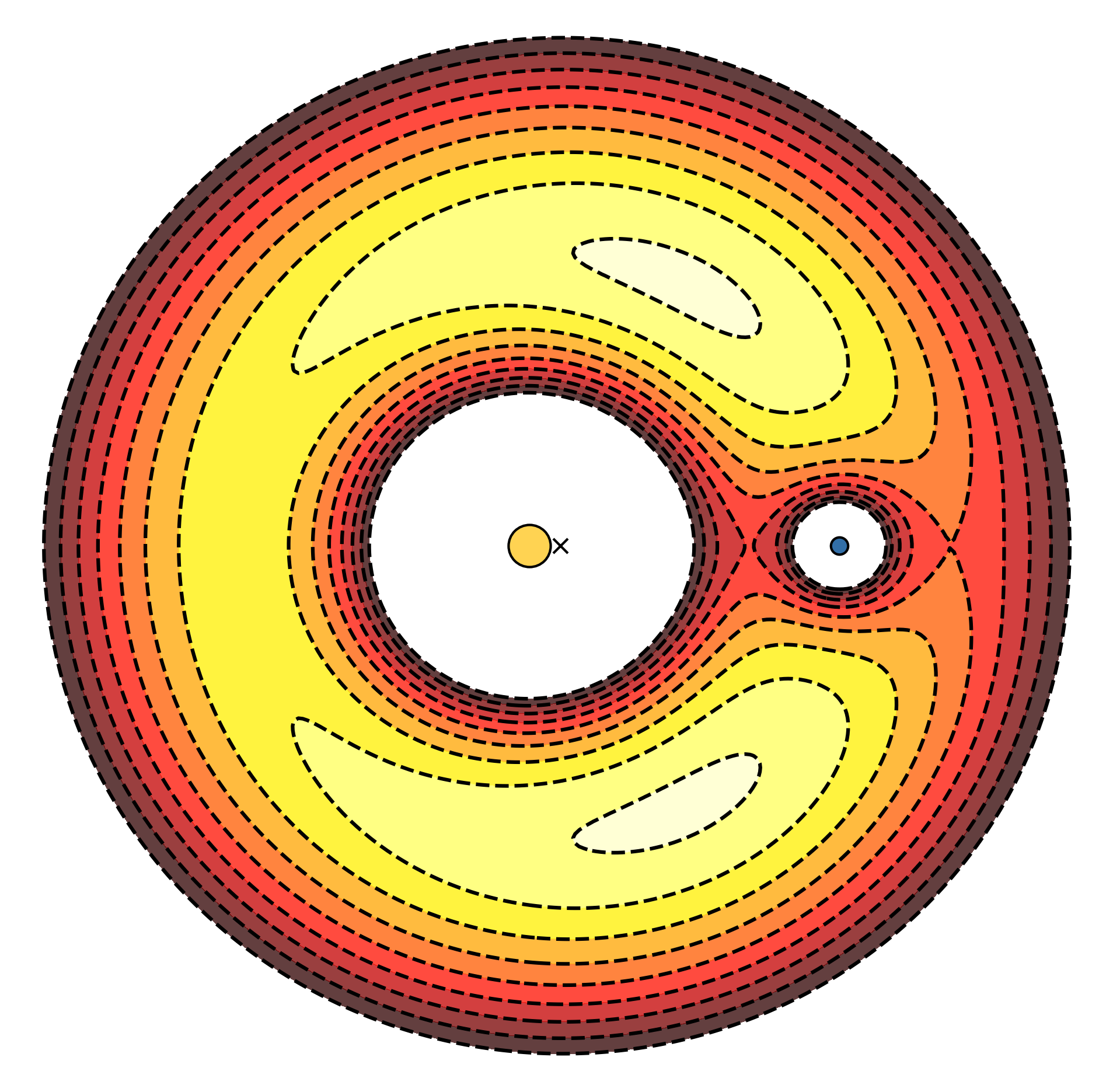
Suppose that we have the sun-earth system. The potential energy of a satellite (any point $(x, y)$ in the system) is determined by the following equation:
$$ u = -\frac{1-\mu}{\sqrt{(x + \mu)^2 + y^2}} - \frac{\mu}{\sqrt{[x - (1 - \mu)]^2 + y^2}} - \frac{1}{2}(x^2 + y^2), $$
where $\mu$ is the distance from the center of rotation (the barycenter).
If we use the equation to create a contour plot, we get a pretty cool visualization of the potential energy in the sun-earth system. The neat thing about this is that you can see the Lagrange points!
The plot has been created with the following Python code:
 1mu = 0.1
 2R = 1
 3sun_pos = np.array([-mu*R, 0])
 4earth_pos = np.array([(1-mu)*R, 0])
 5
 6
 7def f(x, y):
 8    t1 = -(1-mu) / ((x + mu)**2 + y**2)**0.5
 9    t2 = -mu / ((x - (1-mu))**2 + y**2)**0.5
10    t3 = -0.5 * (x**2 + y**2)
11    u = t1 + t2 + t3
12    return u
13
14
15n = 256
16x = np.linspace(-1.75, 1.75, n)
17y = np.linspace(-1.75, 1.75, n)
18X, Y = np.meshgrid(x, y)
19
20plt.figure(figsize=(8, 8))
21levels = np.linspace(-2, -1.4, 10)
22plt.contourf(X, Y, f(X, Y), 8, alpha=.75, cmap=plt.cm.hot, levels=levels)
23C = plt.contour(X, Y, f(X,Y), 2, colors='black', levels=levels)
24plt.scatter(sun_pos[0], sun_pos[1], s=300, c='#ffd352', edgecolor='black')
25plt.scatter(earth_pos[0], earth_pos[1], s=50, c='#326fa8', edgecolor='black')
26plt.scatter(0, 0, marker='x', lw=1, c='black')
27plt.show()