Primer on constraint satisfaction problems

December 7, 2022

A lot of problems can be described as a constraint satisfaction problem (CSP). This post is intended as a short primer to help you get started.

What is a constraint satisfaction problem? #

A constraint satisfaction problem consists of three components. The first component is a variable to which a value can be assigned. The second component is the domain. Each variable has a list of possible values that can be assigned to the variable. This is called the domain of the variable. Usually the domain is the same for all of the variables, but it is also possible that each of the variables have a different domain. The third and last component is a set of constraints. Constraints are used to constrain the values that can be assigned to the variables.

The type of domain that is used for the variables plays a major factor in the approach that is used to solve the problem. If a domain contains a zero and a one, it is called a Boolean domain. Solving constraint satisfaction problems with a Boolean domain is also known as SAT solving, where SAT stands for satisfiability. A domain can also have a discrete set of values, such as red, green, and blue. Usually these are re-encoded as the integers 1, 2, and 3.

A more different type of domain is when there is a range of integers or real numbers. Solving problems with these type of domains requires methods that will not be covered in this post. This post will only look at solving constraint satisfaction problems that have an unordered discrete integer or Boolean domain.

An iconic example #

The most iconic example that is used to explain constraint satisfaction problems is the Australian map coloring problem. The illustration below is a map of Australia and its regions.

The problem is to color each region such that no neighboring region has the same color. This does not seem that difficult, but there is a catch. You are only allowed to use three colors. Now that we have a description of the problem, it is time to formulate this as a constraint satisfaction problem.

Defining the variables #

There are a total of seven different regions that require a color. This tells us that we need to define seven variables, one for each region. This gives us a set of variables, which we will call $\mathcal V$.

$$ \mathcal V = \{ WA, NT, Q, NSW, SA, V, T \} $$

Defining the domains of the variables #

The next thing that we need to do is define the domain of each variable. Because we can only use three colors—red, green, and blue—all of the variables have the same domain. In this example we will not re-encode the colors as an integer, because this keeps the explanation simple. If this is implemented as a program, then it wise to do the re-encoding. Each of the variables has its own domain, $\mathcal D_v$, which is the set

$$ \mathcal D_{v \in \mathcal V} = \{ r, g, b \}. $$

If you have never seen this type of notation, don’t worry. The notation is telling that for each variable $v$ in $\mathcal V$ the domain is defined as $\{ r,g,b\}$. It is defined like this so we can refer to the domain of $SA$ as $\mathcal D_{SA}$.

Defining the constraints of the problem #

The last thing that we need to do is to define the set of constraints $\mathcal C$. To do so, we will create a graph of the map by drawing a node for all of the regions. Two nodes are connected by an edge if they are adjacent regions. This will result in the following graph.

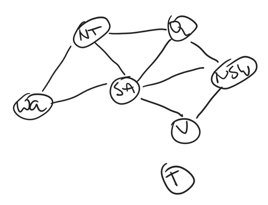
This type of graph is called a constraint graph, and it visualizes how the variables and constraints are related to one another. The constraint that is imposed on the problem says that no adjacent region can have the same color. To formalize this we can define this constraint as a not equal constraint. As an example, $WA$ can not be the same as $NT$, which we can write as

$$ WA \not= NT. $$

If we do this for all the edges in the graph, we get the set $\mathcal C$ which contains the nine constraints

$$ \begin{align} \mathcal C = \{ &WA \not= NT, WA \not= SA, \\ &NT \not= SA, NT \not= Q, \\ &Q \not= SA, Q\not = NSW, \\ &SA \not=NSW, SA\not=V, \\ &NSW \not=V \}. \end{align} $$

Now that the constraints are defined, we have the three components that describe that map coloring problem as a CSP. In the next section we will look at the theory behind solving the problem and in a later section we will implement a program that will find all of the solutions.

How to solve the problem? #

There are a lot of methods that can be used to solve the problem, but we will start with a simple brute force algorithm. Before we can do so, we need to define some terminology.

Terminology #

The domains define what can be assigned to the variables. The search space of the constraint satisfaction problem are all the possible assignments of the variables. This is defined as the Cartesian product of all of the domains, e.g.

$$ \mathcal D_0 \times \mathcal D_1 \times \cdots \times \mathcal D_n. $$

In this specific example there are seven variables and the domain of each variable has three values. This gives a search space that has a total of $3^7 = 2187$ possible configurations. A solution is a configuration that satisfies all of the constraints. An example of a configuration of the map coloring problem is $(r, r, r, r, r, r, r)$, which obviously isn’t a solution to the problem. It is also possible to have a partial configuration, which is a configuration where not all of the variables have been assigned. More specifically, a configuration is an n-tuple, where $n$ is the number of variables in the problem.

We say that a constraint is satisfied if all of the variables have been assigned and the constraint is valid. If not all of the variables have been assigned and the constraint has not been unsatisfied, we say that the constraint is partially satisfied. The scope of a constraint is the set of the variables that are used in the constraint. We say that a constraint is in scope if all of the variables have been assigned.

A brute force approach #

The easiest way—and the most inefficient—to find a solution to the map coloring problem is to generate all the of the configurations and see which of those configurations satisfy all of the constraints. The map coloring problem only has 2187 different configurations so checking all of them easily done on a computer. This problem only has seven variables, but the search space grows with $3^n$, which is exponentially. To generalize this, if we have equal domains of size $d$ and a number of variables $n$, the size of the search space if $d^n$. This quickly becomes a hopeless approach, so what can we do about this?

Search trees #

The search space can be visualized with a search tree. The illustration below shows the search tree of the map coloring problem. This type of visualization is very helpful, because it provides a visual way of thinking about constraint satisfaction problems.

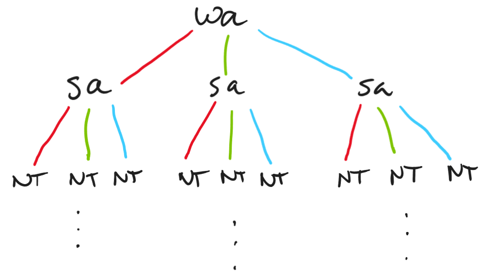
To draw it, start with the first variable. The edges are the possible assignments of that variable, e.g. the values that are in the domain of the variable. At the end of the edge we draw the next variable, with the possible assignments of that variable, and so on. The illustration becomes too big to draw pretty quickly, so usually only the assigned path, or an area of interest, is drawn.

Backtracking #

The key is to check the partial configurations that are generated by the brute force algorithm. Once we find that a partial configuration is violating a constraint, we immediately stop with that partial solution and continue with the next one. As an example: Suppose red is assigned to $WA$. If red is also assigned to $SA$ a constraint is violated. We stop immediately after finding out that it is not possible to assign red to $SA$. The effect of this is that the algorithm prunes all of the configurations that are under that branch of the search tree.

This is already a huge improvement over the brute force approach, but even this method will fail to find a solution in a timely manner for bigger problems. In later posts we will look into techniques that give the much needed performance improvements for solving bigger problems.

Implementation of a backtrack solver #

Enough theory so far! It is time to implement a program that will solve the map coloring problem using the backtracking idea. To do so, we will be using the C# programming language.

The first thing that we need to do is to define a few variables. First we define the number of variables in the problem as N. Then we need to define a mapping of the variables and colors from a name to integers. Finally we will create an array that will store the values that are assigned to the variables.

 1#nullable disable
 2
 3// Number of variables.
 4const int N = 7;
 5
 6// Define all the regions.
 7const int WA = 0, NT = 1, Q = 2, NSW = 3, 
 8          SA = 4, V = 5, T = 6;
 9
10// Define all the domains.
11const int NONE = 0, RED = 1, GREEN = 2, BLUE = 3;
12
13// Used to store the value of the variables.
14var variables = new int[N];

To make it easy to see if we have satisfied all of the constraints, we will add the constraint graph to the program. To do so, we define a helper method EdgeTo which gives a nice descriptive notation about the intention of the code, despite the method doing nothing more than returning the numbers as a list of integers.

1// Helper method to create a list of integers.
2List<int> EdgeTo(params int[] xs) => xs.ToList();

The next thing we will do is use the EdgeTo method to define the constraint graph of the problem as an adjacency list.

 1// Constraint graph of the problem as adjacency list.
 2var edges = new List<int>[N] 
 3{
 4    /* WA  */ EdgeTo(NT, SA),      
 5    /* NT  */ EdgeTo(WA, SA),            
 6    /* Q   */ EdgeTo(NT, SA, NSW),       
 7    /* NSW */ EdgeTo(Q, SA, V),          
 8    /* SA  */ EdgeTo(WA, NT, Q, NSW, V),   
 9    /* V   */ EdgeTo(SA, NSW),            
10    /* T   */ EdgeTo(), 
11};

Now that we know how all of the variables are connected to one and another, we will implement a method that checks if all of the constraints are satisfied. This means that we need to check if all the regions that are adjacent don’t have the same color. A constraint is only checked if it is in scope, or in other words, if all the variables in the constraint have been assigned.

 1// Checks if the constraints are satisfied for 
 2// the assigned variables.
 3bool IsSatisfied()
 4{
 5    for (int i = 0; i < N; i++)
 6        if (variables[i] != NONE)
 7            foreach (int j in edges[i])
 8                if (variables[j] != NONE)
 9                    if (variables[i] == variables[j])
10                        return false;
11    return true;
12}

With all of that in place, we can implement the backtracking method. The idea is to try all of the colors of a variable, and if the assignment is valid, it should go to the next variable. Once it has found a solution, it should stop searching. This can be implemented as a recursive method. First we define the parameter k as the index of the variable that we are currently solving. The base case of the function should return if we have assigned all of the variables. This happens when k is bigger than or equal to the number of variables. The method below is one of the approaches to implement the backtracking algorithm.

 1// Backtrack procedure to enumerate the search space.
 2bool Backtrack(int k = 0) 
 3{
 4    if (k >= N)
 5        return true;
 6
 7    foreach (var color in new int[] { RED, GREEN, BLUE })
 8    {
 9        variables[k] = color; // Assign the color.
10        if (IsSatisfied())
11            if (Backtrack(k + 1)) 
12                return true;
13        variables[k] = NONE; // Unassign the color.
14    }
15
16    return false;
17}

The solution is stored in the array variables after the program has finished. The first solution that it finds to the problem is $(r, g, r, g, b, r, r)$, which we can visually verify to be correct.

By looking at the solution that the algorithm found, we can infer a method to solve the problem ourselves. The region $SA$ is the region that is sharing a border with most other regions. Because of this, starting at this region is usually a very good idea. The idea of starting with the variable that has the most constraints is also known as the most constrained order heuristic. This heuristic is a good method for solving this type of problem quickly.

Another thing that we can think about is what happens if we assign a color a region. If a color is assigned, this means that this color is no longer possible for any adjacent regions. However, the backtracking algorithm does nothing with this information, and is still going to guess something which obviously isn’t possible. The key idea is that if a color is assigned to a region, that color is removed from the domain of all the adjacent regions. This ensures that the backtracking algorithm is not going to guess values of which we already know that they are not. This technique is called forward checking and it is a very powerful! More about this in later post.

Finding all the solutions #

It is also possible to find all of the solution to the map coloring problem with only a minor modification to the algorithm. On line 5, instead of returning true which results in stopping the search procedure, we need to save the solution and return false.

 1List<List<int>> solutions = new();
 2bool Backtrack(int k = 0) 
 3{
 4    if (k >= N)
 5    {
 6        List<int> solution = new();
 7        solution.AddRange(variables);
 8        solutions.Add(solution);
 9        return false;
10    }
11
12    foreach (var color in new int[] { RED, GREEN, BLUE })
13    {
14        variables[k] = color;
15        if (IsSatisfied())
16            if (Backtrack(k + 1)) 
17                return true;
18        variables[k] = NONE;
19    }
20
21    return false;
22}

If we execute the modified backtracking algorithm, it will find a total of 18 different solutions. All the different solutions that is has found are listed below.

 1(1, 2, 1, 2, 3, 1, 1)
 2(1, 2, 1, 2, 3, 1, 2)
 3(1, 2, 1, 2, 3, 1, 3)
 4(1, 3, 1, 3, 2, 1, 1)
 5(1, 3, 1, 3, 2, 1, 2)
 6(1, 3, 1, 3, 2, 1, 3)
 7(2, 1, 2, 1, 3, 2, 1)
 8(2, 1, 2, 1, 3, 2, 2)
 9(2, 1, 2, 1, 3, 2, 3)
10(2, 3, 2, 3, 1, 2, 1)
11(2, 3, 2, 3, 1, 2, 2)
12(2, 3, 2, 3, 1, 2, 3)
13(3, 1, 3, 1, 2, 3, 1)
14(3, 1, 3, 1, 2, 3, 2)
15(3, 1, 3, 1, 2, 3, 3)
16(3, 2, 3, 2, 1, 3, 1)
17(3, 2, 3, 2, 1, 3, 2)
18(3, 2, 3, 2, 1, 3, 3)

Pretty neat huh? It is surprising that out of the 2187 possible configurations, only 18 are a solution to the problem!

What’s next? #

This aim of this post was to give an introductory overview of the basic of constraint satisfaction problems. We looked at the different components of a constraint satisfaction problem and two different algorithms that can be used to solve them. Out of the two algorithms, we created an implementation of the backtracking algorithm, which we used to find all the possible solution to the map coloring problem. This knowlegde should provide a foundation of the terminology and ideas that you will encounter when defining and solving constraint satisfaction problems.

The example that we solved was a very simple example (in CSP terms). In another post we will look at the Sudoku puzzle. Thinking about it, there are 9 different values for 81 squares, this gives a solution space of $9^{81}$ possible configurations. We will see that the backtracking algorithm is not efficient enough to solve this in a timely manner. Instead we will look at other techniques that we will use to solve the puzzle in just a few milliseconds.

Source code #

This is the complete source of the backtracking algorithm that finds a solution to the map coloring problem.

 1#nullable disable
 2
 3// Number of variables.
 4const int N = 7;
 5
 6// Define all the regions.
 7const int WA = 0, NT = 1, Q = 2, NSW = 3, 
 8          SA = 4, V = 5, T = 6;
 9
10// Define all the domains.
11const int NONE = 0, RED = 1, GREEN = 2, BLUE = 3;
12
13// Used to store the value of the variables.
14var variables = new int[N];
15
16// Helper method to create a list of integers.
17List<int> EdgeTo(params int[] xs) => xs.ToList();
18
19// Constraint graph of the problem as adjacency list.
20var edges = new List<int>[N] 
21{
22    /* WA  */ EdgeTo(NT, SA),      
23    /* NT  */ EdgeTo(WA, SA),            
24    /* Q   */ EdgeTo(NT, SA, NSW),       
25    /* NSW */ EdgeTo(Q, SA, V),          
26    /* SA  */ EdgeTo(WA, NT, Q, NSW, V),   
27    /* V   */ EdgeTo(SA, NSW),            
28    /* T   */ EdgeTo(), 
29};
30
31// Checks if the constraints are satisfied for 
32// the assigned variables.
33bool IsSatisfied()
34{
35    for (int i = 0; i < N; i++)
36        if (variables[i] != NONE)
37            foreach (int j in edges[i])
38                if (variables[j] != NONE)
39                    if (variables[i] == variables[j])
40                        return false;
41
42    return true;
43}
44
45// Backtrack procedure to enumerate the search space.
46bool Backtrack(int k = 0) 
47{
48    if (k >= N)
49        return true;
50
51    foreach (var color in new int[] { RED, GREEN, BLUE })
52    {
53        variables[k] = color; // Assign the color.
54        if (IsSatisfied())
55            if (Backtrack(k + 1)) 
56                return true;
57        variables[k] = NONE; // Unassign the color.
58    }
59
60    return false;
61}
62
63// Solve the puzzle.
64Backtrack();
65Console.WriteLine($"({string.Join(", ", variables)})");