Iterated function systems

December 22, 2020

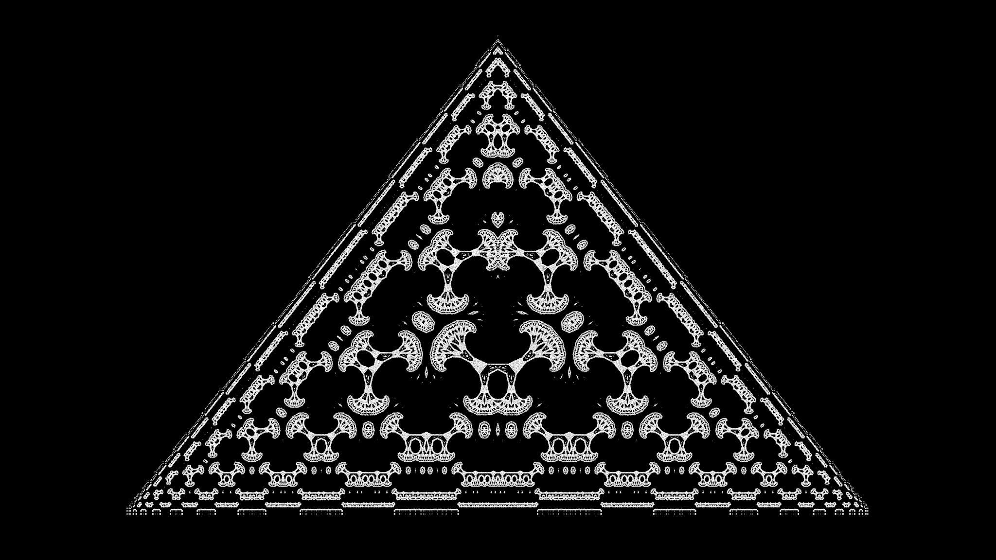
In this post I will explain a simple iterated function system, also called IFS. We will start of with explaining the basic transformations that we apply, and finally work our way up to get a result like this.

I have also included a live demo below that is hosted on ShaderToy. Click play to run the shader. You can change the scaling parameter with the $y$ value of the mouse, and the rotation parameter can be changed with the $x$ value of the mouse. If the mouse is not pressed, it will animate the rotation parameter.

The basic transformations

To really see what is going on, and how the coordinate system is transformed, I grabbed a shader that renders a grid, unit square, and the axis. I removed the Mobius transformation, and centered it, which results in this.

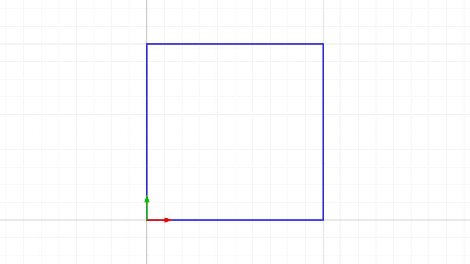
The first transformation we will apply is the abs() function, and apply this only to the x-axis.

uv.x = abs(uv.x);

If we apply the abs() function, it will map all the negative values, to positive values. This results in a copy of the unit square, as seen in the image below.

Coordinate space with abs() applied to the x-axis.

It is worthwhile to note that we haven't changed anything to draw this. This is simply the result of feeding the transformed coordinate space through the same drawing function. If we would draw a circle at $(0.5, 0.5)$, it will also show up on the "negative" side, because the coordinates there are exactly the same as on the right side.

The next transformation that we will apply is a translation. We will move the unit square, one unit to the right.

uv -= vec2(1, 0);

After we have applied this transformation, the coordinate space looks like this.

Coordinate space after translating unit square to the right.

Before we translated the coordinate space, both of the axis were located at the point $(0, 0)$. If we would draw a circle at $(0, 0)$, we would only get one circle, because they are overlapping each other at the same place. After the translation, we now have two points for $(0, 0)$, and if we then draw a circle, we would get two of them!

Now we are going to add another transformation. We are going to rotate the coordinate space by $90$ degrees. Later on we will want to rotate it by any angle, but let's keep it simple for now. Rotating by $90$ degrees can be done with $(x, y) \rightarrow (-y, x)$.

uv.xy = uv.yx;
  uv.y = -uv.y;

After applying the rotation transformation, the coordinate space looks like this.

Coordinate space after a rotation by $90$ degrees.

There is nothing special about rotating it by $90$ degrees, actually it produces the most boring result. Most of the complex shapes emerge when we use a rotation that is different than $90$, $180$, or $270$ degrees. However, I chose $90$ degrees here, so we can see how the coordinate space changes while we are still creating the IFS.

Finally, we are going to scale everything by $1.25$. This is also a good parameter that we are going to use later, but this will do for now.

uv *= 1.25;

After we have applied the scaling transformation, the final result of all our transformations looks like this.

So far we have mapped the negative values to positive values, added a translation, added a rotation, and scaled the coordinate space. These are the four basic transformations that are used to create the IFS.

Now let's iterate

The key trick is when we repeatedly apply these transformations. We are going to wrap the transformations in a for loop, and to easily use it, we will also put them in a function.

vec2 ifs(vec2 uv, int n) {
      for(int i=0; i < n; i++) {
          uv.x = abs(uv.x);  // Map negative to positive
          uv -= vec2(1, 0);  // Translate to the right
          uv.xy = uv.yx;     // Rotate 90 degrees
          uv.y = -uv.y;
          uv *= 1.25;
      }
      return uv;
  }

Let's see what this function does by setting $n$ to $2$, $3$, and $4$. I have included the images below.

Coordinate space after applying ifs(uv, 2).

Coordinate space after applying ifs(uv, 3).

Coordinate space after applying ifs(uv, 4).

We can see that each time all these transformations are iterated, we create an entire copy of the previous coordinate space. Cool! Now instead of drawing the grid, unit square, and axis, let's draw a circle at $(0, 0)$ with a radius of $0.5$.

Drawing a circle at $(0, 0)$ after applying ifs(uv, 4).

Although we are now finally having an image, this result isn't really that interesting. Let's try and see what we will get if we set $n$ to $12$.

Drawing a circle at $(0, 0)$ after applying ifs(uv, 12).

Wonderful, we have created even more circles. This still doesn't look anything like the demo in the beginning of the post, but trust me, we are almost there.

Playing with parameters

The real fun begins when we are going to change the rotation and scaling parameters. To easily do this, we will modify the ifs(uv, n) function to also accept a rotation $r$, and a scale $s$.

vec2 ifs(vec2 p, float s, float r, int n) {
      float co = cos(r), si = sin(r);
      mat2 rot = mat2(co, si, -si, co);
      for(int i=0; i < n; i++) {
          p.x = abs(p.x);
          p -= vec2(1.0, 0);
          p *= rot;
          p *= s;
      }
      return p;
  }

If we now apply the ifs(uv, s, r, n) function with the scale set to $1.11$, the rotation set to $\frac{\pi}{2}$, and $n=32$, we get this square.

Image of ifs(uv, 1.11, pi/2, 32).

However, if we now use different angles instead of $90$ degrees, we will get much more interesting results. Here are three images where we use different angles. The first images uses an angle of $0.39$ radians.

Image of ifs(uv, 1.11, 0.39, 32).

If we set the ange to $\frac{\pi}{3}$, we get a hexagon structure with Sierpinski triangles in it.

Image of ifs(uv, 1.11, 1.046, 32).

If the angle is $\pi$ we get a straight line, which is not that interesting. But if we add a little bit to it we get these tree shapes.

Image of ifs(uv, 1.11, 3.38, 32).

Of course I can imagine that you would like to see other angles too. I included a shader below where you can use the $x$ value of the mouse to select an angle between $[0, 2\pi]$. If the mouse is not used, it will animate the angle. Click play to animate the shader.

Another thing we can do to change the appearance is by changing the radius of the circle. In the shader that is used as the demo the radius is set to $0.8$. The demo also has antialiasing added to it, which is why it looks better than the examples we have created earlier.

You also might have noticed that the translation is set to vec2(1, 0). This is another parameter that we can use to change the appearance of the IFS. I left this as something that can be implemented by the reader.

Behind the scenes

To get some more insight into what is happening, we are going back to displaying the coordinate space, and see how it transforms when the angle or scale is changed. The examples below is are renders of ifs(uv, mouse y, mouse x, n) where $n$ is set to $1$, $2$, and $4$. Again, you can use the mouse here to play with the parameters, and otherwise they will be animated.

I find it rather hard to describe what is going on here, but I included them because they show a unique aspect of what is happening to the coordinate spaces.

More images

Image of ifs(ifs(uv, 1.11, PI/3, 24), 1.17, PI/2, 8).

Image of ifs(ifs(uv, 1.11, 3PI/4, 24), 1.17, PI/2, 8).

Image of ifs(ifs(uv, 1.11, 0.47, 24), 1.17, PI/2, 8).

Image of ifs(ifs(uv, 1.11, 1.94, 24), 1.17, PI/2, 8).