Monopoly odds

February 28, 2021

Introduction #

A few years ago I have written a detailed analysis of the probabilities in Monopoly. However, because of handwaving many rules to make it easier to analyze, I wanted to redo it and use all the rules this time. The main motivation for doing this is to solve a question on Project Euler. While we are at it, I also wanted to take the time to answer a few different questions as well. I will assume that the rules of Monopoly are known to you, and will only describe the rules which we are going to use in this model.

There are two methods that we can use to find the probabilities that a player can land on each cell. We can use a Monte carlo method, where we will simply simulate the game for a large number of rounds, and track how many times each cell is visited. However, a more accurate result is given by the steady state vector of a Markov matrix, which is the method I’m going to use.

In the first section we will look at what a Markov matrix is, and how to find the steady state vector. Then we are going to translate the Monopoly rules into a Markov process, and find the steady state vector. Finally, we are going to analyze the results, and solve the Project Euler problem.

What is a Markov process? #

A Markov proces is a proces where we have different states, and a probability to move between each state. If we use the weather as a simple example, we will have two states: sunny or rainy. This markov process can be illustrated by drawing a graph in the following way:

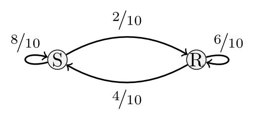
We can see that if it is sunny, there is a probability of $80\%$ that it will stay sunny, and a probability of $20\%$ that it is going to rain. We can use this to answer questions like, what is the probability that the sun will shine seven consecutive days, given that today is sunny? To find this probability we know that we have to transition from $S \rightarrow S$, seven times in a row, which gives us a probability of $\left(\frac{8}{10}\right)^7 \approx 0.2097$. There is a probability of approximately $21\%$ that the sun will shine for an entire week.

However, to answer a question like “Which percentage of days in a year does the sun shine?”, requires us to take things a bit further. Perhaps you have noticed, but this question is exactly the same as “What is the probability that each cell is visited by a player in a game of Monopoly?” in Markov terms.

The transition matrix #

The first thing we are going to do, is to describe the Markoc proces as a transition matrix. The transition matrix for the weather example will look like this:

$$ \mathbf{M} = \begin{bmatrix} \frac{8}{10} \frac{2}{10} \ \frac{4}{10} \frac{6}{10} \ \end{bmatrix} $$

If we have this matrix $\mathbf{M}_{ij}$, then each entry can be read as the probability to move from state $i$ to state $j$. Any matrix that has the following two properties is a Markov matrix:

1. The sum of all the elements in a row is $1$.
2. Every entry in the matrix is $\geq 0$.

Once we have determined that a matrix is a Markov matrix, we can use many of the theorems and properties that apply to Markov matrices. One of these properties is that the transition matrix has a steady state vector. This steady state vector will tell us the percentage of rainy days over a long period of time, or the probability that a player is on a given cell over many games of Monopoly. In essence, it tells us the long term behaviour of the Markov process.

How to find the steady state vector? #

The steady state vector of a matrix is the vector $\pi$ (this has nothing to do with the number $\pi$) such that $\pi\mathbf{M} = \pi$, meaning that if we multiply the steady state vector by the transition matrix, we get the steady state vector back. In the case of our weather example, the steady state vector is $\pi = \begin{bmatrix}\frac{2}{3} & \frac{1}{3}\end{bmatrix}$, or any scaled version of $\pi$, as long as the ratio is the same. The zero vector doesn’t count. The example below will verify that it is indeed the steady state vector.

Input

1M = np.mat([[8/10, 2/10], [4/10, 6/10]])
2x = np.mat([2/3, 1/3])
3x * M

Output

matrix([[0.66666667, 0.33333333]])

As you can see, the result is the same as the vector $\pi$, which means that this is indeed the steady state vector. But how do we find this steady state vector? Suppose we will begin on a sunny day. We can describe this initial condition with the vector $\pi_0 = \begin{bmatrix}1 & 0\end{bmatrix}$. If we multiply $\pi_0$ with the transition matrix $\mathbf M$, we will get the probabilities of each state at day $1$:

Input

1x = np.mat([1, 0])
2x * M

Output

matrix([[0.8, 0.2]])

This gives the state with the probabilities that we are in a certain state after one day. It says that we have a probability of $20\%$ that it will rain. If we multiply this by $\mathbf M$ again, we will get the probabilites of each state on day 2.

Input

1np.matrix([[0.8, 0.2]]) * M

Output

matrix([[0.72, 0.28]])

On day 2 there is a probability of $28\%$ that it will rain. We can keep doing to this to find the probability up to day $n$. However, there is an easier method that we can use.

First let us continue this process, and write out the consecutive steps in the following way:

$$ \begin{align} \pi_0 &= \begin{bmatrix}1 & 0\end{bmatrix} \\ \pi_1 &= \pi_0\cdot\mathbf M \\ \pi_2 &= \pi_1\cdot\mathbf M \\ \pi_3 &= \pi_2\cdot\mathbf M \\ \end{align} $$

If we now substitute $\pi_2$ backwards, we will get:

$$ \begin{align} \pi_3 &= \pi_2\cdot\mathbf M \\ \pi_3 &= (\pi_1\cdot\mathbf M)\cdot\mathbf M \\ \pi_3 &= ((\pi_0\cdot\mathbf M)\cdot\mathbf M)\cdot\mathbf M \\ \pi_3 &= \pi_0\cdot\mathbf M\cdot\mathbf M\cdot\mathbf M \\ \pi_3 &= \pi_0\cdot\mathbf M^3 \\ &\vdots \\ \pi_n &= \pi_0\cdot\mathbf M^n \end{align} $$

Which is a rather useful result. Instead of finding $\pi_n$ by multiplying $\pi_{n-1}\cdot\mathbf M$, we can also raise $\mathbf M$ to the $n$-th power to get the probabilities on day $n$. As more days pass, and $n \rightarrow\infty$, this will converge to the steady state vector. This means that we can find the steady state vector with

$$ \pi = \lim\limits_{n\rightarrow\infty} \pi_0\cdot\mathbf M^n. $$

We can easily verify this by calculating $\mathbf M$ for a high power.

Input

1x * M**32

Output

matrix([[0.66666667, 0.33333333]])

Which is the steady state vector! In this example the steady state vector tells us that:

• $\frac{2}{3}$ of the time the weather is sunny,
• $\frac{1}{3}$ of the time it rains.

However, there is another method we can use to find the steady state vector.

Eigenvectors and the steady state vector #

If we calculate the eigenvalues and eigenvectors of the transpose of $\mathbf M$.

Input

1eigenvalues, eigenvectors = eig(M.T)
2eigenvalues.real

Output

array([1. , 0.4])

Input

1eigenvectors

Output

array([[ 0.89442719, -0.70710678],
       [ 0.4472136 ,  0.70710678]])

We want to use the eigenvector where the corresponding eigenvalue is $1$. In this case it is the first column vector of the matrix of eigenvectors. You might notice that this doesn’t look like our steady state vector at all, but if we multiply this eigenvector with $\mathbf M$, we will see that it is correct.

Input

1eigenvectors.T[0] * M

Output

matrix([[0.89442719, 0.4472136 ]])

If we normalize the eigenvector, it becomes immediately obvious that this is our steady state vector.

Input

1x = eigenvectors.T[0]
2x / sum(x)

Output

array([0.66666667, 0.33333333])

Nice! Now that we have a method to find the steady state vector of a transition matrix, we can start to create the transition matrix for the Monopoly model.

Monopoly as a Markov process #

Before we can create the transition matrix for the game of Monopoly, we will first have to determine which of the rules which we are going to include in the model. First, let’s take a look at the game board:

Because we want to use the result to solve the Project Euler question, we will use the rules that are defined in the problem statement.

• There are a total of 40 cells, which we will label as $c_0, c_1, \ldots, c_{39}$.
• We will throw with two dices that have four sides. However, we also want to be able to use six sides (the traditional method).
• If we throw a double, the player can throw again. However, if three consecutive doubles are rolled, the player moves directly to jail.
• There are chance cards CC, and community chest cards CH which moves the player, thus having an impact on the probability distribution.

Now that we have defined the rules, we can start to model them as a Markov process.

Probability distribution of throwing two dice #

If we throw a single dice, we have a uniform probability to get each side. However, when two dice are used, the probability distribution is different. In this case it is the sum of two uniform probability distributions. The following table shows the sum of throwing two dice:

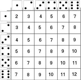
If we let $\underline{k}$ be a random stochast of throwing two dice with six sides, then we can see from the table that $P(\underline{k} = 2) = \frac{1}{36}$ because there is only one possible way of obtaining the sum of $2$ out of the $36$ possible outcomes. In the case of $P(\underline{k} = 7)$, we can see that there are $6$ possible outcomes, which gives the probability of $\frac{6}{36}$.

Encoding the probability distribution in a vector #

We are going to encode the probability distribution as a vector with $40$ elements. The first element will correspond with $c_0$, which is GO, all the way up to $c_{39}$. Starting at $c_0$, we will calculate the probability of landing on each square. We only have to calculate this distribution vector for the starting position $c_0$. If the player is not at $c_0$, but on another cell, we can simply shift the vector while wrapping, which we can do with np.roll(...). Let’s start by defining a few functions to create this vector.

1def cross_sum(S):
2  return [(a + b) for a in S for b in S]

We can use this function to obtain all the possible outcomes for a set $S$, which in the case of a four side dice is ${1, 2, 3, 4}$.

Input

1cross_sum(range(1, 4 + 1))

Output

[2, 3, 4, 5, 3, 4, 5, 6, 4, 5, 6, 7, 5, 6, 7, 8]

Next, we are going to create this vector with $40$ elements, and count how many times we land on each cell. Finally, we divide the entire vector by the total number of outcomes to get the probabilities. Notice that the sum of all the elements in this vector is $1$, which is a requirement of the transition matrix.

1def two_dice_distribution(num_sides):  
2  outcomes = cross_sum(range(1, num_sides+1))
3  D = np.array([0] * 40)
4  for outcome in outcomes:
5    D[outcome] += 1
6  D = 1 / (num_sides * num_sides) * D
7  return D

If we then test this method with dices that have four sides.

Input

1two_dice_distribution(4)

Output

array([0.    , 0.    , 0.0625, 0.125 , 0.1875, 0.25  , 0.1875, 0.125 ,
       0.0625, 0.    , 0.    , 0.    , 0.    , 0.    , 0.    , 0.    ,
       0.    , 0.    , 0.    , 0.    , 0.    , 0.    , 0.    , 0.    ,
       0.    , 0.    , 0.    , 0.    , 0.    , 0.    , 0.    , 0.    ,
       0.    , 0.    , 0.    , 0.    , 0.    , 0.    , 0.    , 0.    ])

Constructing the transition matrix #

To construct the transition matrix, we need to create this distribution vector for each cell $c_n$. We do this by creating the distribution vector starting at $c_0$, and then shift it by $n$, to get the distribution vector for $c_n$. If we repeat this for every cell, this will give us a total of $40$ vectors, which we are going to use as the rows to construct the transition matrix.

We will also add a placeholder method, in which we will later add the rules for double throws.

1def dice_distribution(cell_index, num_sides):
2  distribution = two_dice_distribution(num_sides)
3  distribution = np.roll(distribution, cell_index)
4  # TODO: add other rules
5  return distribution

Finally, we will construct the transition matrix by creating $40$ distribution vectors for each cell, and use them as the rows in the transition matrix.

1def monopoly_transition_matrix(num_sides):
2  rows = []
3  for i in range(40):
4    distribution = dice_distribution(i, num_sides)
5    rows.append(distribution)
6  return np.matrix(rows)

Let’s test this function and see what this matrix looks like.

Input

1M = monopoly_transition_matrix(6)
2plt.matshow(M, cmap="inferno")
3plt.colorbar()
4plt.ylabel("Source")
5plt.xlabel("Target")

Output

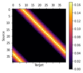
This looks OK. We can also look at the steady state vector of this matrix, using the eigenvector method.

Input

1eigenvalues, eigenvectors = eig(M.T)
2steady_state = eigenvectors.T[0].real
3steady_state /= sum(steady_state)
4steady_state

Output

array([0.025, 0.025, 0.025, 0.025, 0.025, 0.025, 0.025, 0.025, 0.025,
       0.025, 0.025, 0.025, 0.025, 0.025, 0.025, 0.025, 0.025, 0.025,
       0.025, 0.025, 0.025, 0.025, 0.025, 0.025, 0.025, 0.025, 0.025,
       0.025, 0.025, 0.025, 0.025, 0.025, 0.025, 0.025, 0.025, 0.025,
       0.025, 0.025, 0.025, 0.025])

This tells us that the probability to land on each cell is $2.5\%$, which agrees with what is described in the problem statement for the problem on Project Euler.

Implementing cards and other cases #

Now that we have a basic transition matrix for a single roll of two dices, we can implement the chance and community chest cards. First let’s recall what all the possible outcomes are.

• Chance cards (2/16 cards)
  1. Advance to GO.
  2. Go to JAIL.
• Community chest cards (10/16 cards)
  1. Advance to GO.
  2. Go to JAIL.
  3. Go to C1.
  4. Go to E3.
  5. Go to H2.
  6. Go to R1.
  7. Go to next R (railway company)
  8. Go to next R.
  9. Go to next U (utility company)
  10. Go back $3$ squares.

To conveniently use the labels of the board, we will first declare all the different cells as an integer, and a list to find the corresponding label for a cell number.

 1GO = 0; A1 = 1; CC1 = 2; A2 = 3; T1 = 4; R1 = 5; B1 = 6; CH1 = 7; B2 = 8; 
 2B3 = 9; JAIL = 10; C1 = 11; U1 = 12; C2 = 13; C3 = 14; R2 = 15; D1 = 16; 
 3CC2 = 17; D2 = 18; D3 = 19; FP = 20; E1 = 21; CH2 = 22; E2 = 23; E3 = 24; 
 4R3 = 25; F1 = 26; F2 = 27; U2 = 28; F3 = 29; G2J = 30; G1 = 31; G2 = 32; 
 5CC3 = 33; G3 = 34; R4 = 35; CH3 = 36; H1 = 37; T2 = 38; H2 = 39
 6
 7labels = ['GO', 'A1', 'CC1', 'A2', 'T1', 'R1', 'B1', 'CH1', 'B2', 'B3', 
 8          'JAIL', 'C1', 'U1', 'C2', 'C3', 'R2', 'D1', 'CC2', 'D2', 'D3', 
 9          'FP', 'E1', 'CH2', 'E2', 'E3', 'R3', 'F1', 'F2', 'U2', 'F3', 
10          'G2J', 'G1', 'G2', 'CC3', 'G3', 'R4', 'CH3', 'H1', 'T2', 'H2']

Case 1 — Chance cards #

Looking at the two different type of cards, we find the following probabilities:

• Advance to GO is $P(CC = \textrm{GO}) = \frac{1}{16}$.
• Go to JAIL is $P(CC = \textrm{JAIL}) = \frac{1}{16}$.
• A probability of $\frac{14}{16}$ to not move.

Because there are three cells: CH1, CH2, and CH3, we have to redistribute the probabilities for these cells. Let’s look at an example. The probability that we land in jail, is the probability that we land on the chance card multiplied by the probability that we pick the go to jail card. Suppose the probability that we land on CH4 is $10\%$. This will then give $10\%\cdot\frac{1}{16} = 0.625\%$ as a result.

1def apply_chance_card(x):
2  for CC in [CC1, CC2, CC3]:
3    p_cc = x[CC]
4    x[CC] *= 14 / 16
5    x[GO] += 1 / 16 * p_cc
6    x[JAIL] += 1 / 16 * p_cc

We can now apply this function to the probability distribution for any $c_n$, and it will redistribute the probabilities. If the probability to land on the chance card is $0\%$ to begin with, then nothing will be redistributed.

1def dice_distribution(cell_index, num_sides):
2  distribution = two_dice_distribution(num_sides)
3  distribution = np.roll(distribution, cell_index)
4  apply_chance_card(distribution)
5  return distribution

Let’s quickly test this by checking if the probability to land on JAIL has increased.

Input

1M = monopoly_transition_matrix(6)
2eigenvalues, eigenvectors = eig(M.T)
3steady_state = eigenvectors.T[0].real
4steady_state /= sum(steady_state)
5steady_state[JAIL]

Output

0.02946038636979632

Which has indeed been increased to approximately $2.9\%$.

Case 2 — Community chest cards #

Because there are quite a few more community chest cards that have an impact on the probability distribution, implementing this one takes more time. Let’s start with creating a dictionary that helps us to find the correct railway and utility companies.

1nearest_railway = {CH1: R2, CH2: R3, CH3: R1}
2nearest_utility = {CH1: U1, CH2: U2, CH3: U1}

Here we use the same approach as with the chance cards, except it is easier here to store all the other cards in a list. We can then remove the probability from the CH cell, iterate over all the cards and then distribute the probabilities to the cells.

 1def apply_community_chest_card(x):
 2  for CH in [CH1, CH2, CH3]:
 3    p_ch = x[CH]
 4    x[CH] *= 6/16
 5    cards = [GO, JAIL, C1, E3, H2, R1, CH-3, 
 6             nearest_railway[CH], 
 7             nearest_railway[CH], 
 8             nearest_utility[CH]]
 9    for card in cards:
10      x[card] += 1/16 * p_ch

Again, we will add this function to the dice_distribution function.

1def dice_distribution(cell_index, num_sides):
2  distribution = two_dice_distribution(num_sides)
3  distribution = np.roll(distribution, cell_index)
4  apply_chance_card(distribution)
5  apply_community_chest_card(distribution)
6  return distribution

We can quickly test this by confirming that the sum of every row is $1$.

Input

1M = monopoly_transition_matrix(6)
2M.sum(axis=1).T

Output

matrix([[1., 1., 1., 1., 1., 1., 1., 1., 1., 1., 1., 1., 1., 1., 1., 1.,
         1., 1., 1., 1., 1., 1., 1., 1., 1., 1., 1., 1., 1., 1., 1., 1.,
         1., 1., 1., 1., 1., 1., 1., 1.]])

Which it is indeed!

Case 3 — Go to jail #

At this moment, G2J is still considered as a cell, however, the probabilities of G2J have to be added to JAIL because you can’t end up at G2J. Implementing this is rather straightforward.

1def apply_go_to_jail(x):
2  x[JAIL] += x[G2J]
3  x[G2J] = 0

Again, we will add this to the dice_distribution function.

1def dice_distribution(cell_index, num_sides):
2  distribution = two_dice_distribution(num_sides)
3  distribution = np.roll(distribution, cell_index)
4  apply_chance_card(distribution)
5  apply_community_chest_card(distribution)
6  apply_go_to_jail(distribution)
7  return distribution

With almost all the rules applied, let’s take another look at how the transition matrix looks.

Input

1M = monopoly_transition_matrix(6)
2plt.matshow(M, cmap="inferno")
3plt.colorbar()
4plt.ylabel("Source")
5plt.xlabel("Target")

Output

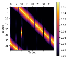
The effect of this rule is pretty visible, all the probabilities from row $30$ (G2J) have been moved to row $10$ (JAIL). We can also clearly see where the community chest cards are.

Solving the Project Euler question #

The questions asks us to concatenate the cell numbers for the three cells which have the highest probability to land on. As a method to verify our work, the question has included the answer for throwing with 6-sided dices. In this case, the answer is 102400.

Verifying the given solution #

Let’s see if our method gives the same result.

First we will create the transition matrix for 6-sides dices.

1M = monopoly_transition_matrix(6)

Then we are going to calculate the steady state vector for the transition matrix.

1eigenvalues, eigenvectors = eig(M.T)
2steady_state = eigenvectors.T[0].real
3steady_state /= sum(steady_state)

Once we have the steady state vector, we create a list of tuples with the probability to land on the cell, and the cell number.

Input

1cells = [(p, i) for i, p in enumerate(steady_state)]
2cells[:3]

Output

[(0.031073154066202282, 0),
 (0.021547417364822227, 1),
 (0.019013909910947927, 2)]

Finally we can sort this in descending order with the sorted(…) function, select the first three tuples, and concatenate them into the correct string.

Input

1"".join([str(c).rjust(2, '0') for _, c in sorted(cells, reverse=True)[:3]])

Output

102400

Awesome, we have found the correct result, which validates that our method is correct.

Finding the solution #

Now we simple change the number of sides for the dices to four to find the answer to the problem.

Input

1M = monopoly_transition_matrix(4)
2eigenvalues, eigenvectors = eig(M.T)
3steady_state = eigenvectors.T[0].real
4steady_state /= sum(steady_state)
5cells = [(p, i) for i, p in enumerate(steady_state)]
6cells[:3]
7"".join([str(c).rjust(2, '0') for _, c in sorted(cells, reverse=True)[:3]])

Output

****** // Solution redacted

Which tells us that ****** is the answer to the problem. If we use this as the solution to the question, Project Euler indeed verifies that this is correct! Pfew, that was quite some work, but we have solved the question!

OK, I have to admit that I cheated a little. I tried to find the solution before applying the rules of double throwing. To my surprise, the answer was correct! However, the same result is found if we apply the rules for double throwing, which in my opinion makes the model more accurate, although the error might be negligible.

Complete source code #

This is the complete source code that will print the solution.

 1import numpy as np
 2from scipy.linalg import eig
 3
 4GO = 0; A1 = 1; CC1 = 2; A2 = 3; T1 = 4; R1 = 5; B1 = 6; CH1 = 7; B2 = 8; 
 5B3 = 9; JAIL = 10; C1 = 11; U1 = 12; C2 = 13; C3 = 14; R2 = 15; D1 = 16; 
 6CC2 = 17; D2 = 18; D3 = 19; FP = 20; E1 = 21; CH2 = 22; E2 = 23; E3 = 24; 
 7R3 = 25; F1 = 26; F2 = 27; U2 = 28; F3 = 29; G2J = 30; G1 = 31; G2 = 32; 
 8CC3 = 33; G3 = 34; R4 = 35; CH3 = 36; H1 = 37; T2 = 38; H2 = 39
 9
10labels = ['GO', 'A1', 'CC1', 'A2', 'T1', 'R1', 'B1', 'CH1', 'B2', 'B3', 
11          'JAIL', 'C1', 'U1', 'C2', 'C3', 'R2', 'D1', 'CC2', 'D2', 'D3', 
12          'FP', 'E1', 'CH2', 'E2', 'E3', 'R3', 'F1', 'F2', 'U2', 'F3', 
13          'G2J', 'G1', 'G2', 'CC3', 'G3', 'R4', 'CH3', 'H1', 'T2', 'H2']
14
15def cross_sum(S):
16  return [(a + b) for a in S for b in S]
17
18def two_dice_distribution(num_sides):  
19  outcomes = cross_sum(range(1, num_sides+1))
20  D = np.array([0] * 40)
21  for outcome in outcomes:
22    D[outcome] += 1
23  D = 1 / (num_sides * num_sides) * D
24  return D
25
26def apply_chance_card(x):
27  for CC in [CC1, CC2, CC3]:
28    p_cc = x[CC]
29    x[CC] *= 14 / 16
30    x[GO] += 1 / 16 * p_cc
31    x[JAIL] += 1 / 16 * p_cc
32
33nearest_railway = {CH1: R2, CH2: R3, CH3: R1}
34nearest_utility = {CH1: U1, CH2: U2, CH3: U1}
35
36def apply_community_chest_card(x):
37  for CH in [CH1, CH2, CH3]:
38    p_ch = x[CH]
39    x[CH] *= 6/16
40    cards = [GO, JAIL, C1, E3, H2, R1, CH-3, 
41             nearest_railway[CH], 
42             nearest_railway[CH], 
43             nearest_utility[CH]]
44    for card in cards:
45      x[card] += 1/16 * p_ch
46
47def apply_go_to_jail(x):
48  x[JAIL] += x[G2J]
49  x[G2J] = 0
50
51def dice_distribution(cell_index, num_sides):
52  distribution = two_dice_distribution(num_sides)
53  distribution = np.roll(distribution, cell_index)
54  apply_chance_card(distribution)
55  apply_community_chest_card(distribution)
56  apply_go_to_jail(distribution)
57  return distribution
58
59def monopoly_transition_matrix(num_sides):
60  rows = []
61  for i in range(40):
62    distribution = dice_distribution(i, num_sides)
63    rows.append(distribution)
64  return np.matrix(rows)
65
66M = monopoly_transition_matrix(6)
67eigenvalues, eigenvectors = eig(M.T)
68steady_state = eigenvectors.T[0].real
69steady_state /= sum(steady_state)
70cells = [(p, i) for i, p in enumerate(steady_state)]
71"".join([str(c).rjust(2, '0') for _, c in sorted(cells, reverse=True)[:3]])