Projectile motion (part I)

November 19, 2022

In this post we will be looking at the motion of projectiles. Starting from first principles by deriving the equations governing projectile motion. In a later post we will be studying how the different quantities are related.

Deriving the equations #

A projectile is an object which is moving over time because of its velocity and acceleration. As we know from physics, components that are perpendicular behave independently. In our 2D case this means that the horizontal and vertical components of motion are independent of each other. Any motion in the horizontal direction does not affect the motion in the vertical direction and vice versa.

Acceleration #

We will start by defining a model where only gravity, denoted by $g$, is excerting force on the projectile. Starting from first principles, this means that there is a downward acceleration on the projectile. Let $\mathbf a(t)$ be the acceleration at time $t$, which we define as

$$ \mathbf a(t) = - g \cdot \mathbf { \hat j }, \tag{1} $$

where $\mathbf {\hat j}$ is the unit vector in the y-direction. This is a constant function, which does not depend on $t$ in any way. The force of gravity is constant at any point in time.

Velocity #

To get the velocity, denoted as $\mathbf v(t)$, we need to integrate the acceleration with respect to $t$, giving the indefinite integral

$$ \int \mathbf a(t)\ dt = \int -g \cdot \mathbf { \hat j } \ dt $$

which results in

$$ \mathbf v(t) = - g t \cdot \mathbf {\hat j} + C. $$

Note that the constant of integration $C$ is equal to the velocity at $t=0$, denoted as $\mathbf v(0)$, giving the function of the velocity

$$ \mathbf v(t) = \mathbf v(0) -g t \cdot \mathbf {\hat j} \tag{2} $$

The gravitational force now is depending on $t$. As time progresses, the gravitational force increases the projectile’s velocity linearly.

Displacement #

To get the displacement of the projectile, denoted as $\mathbf d(t)$, we need to integrate the velocity, yet again with respect to $t$.

$$ \int \mathbf v(t)\ dt = \int \left( \mathbf v(0) - g t \cdot \mathbf {\hat j} \right)\ dt, $$

which results in

$$ \mathbf d(t) = t \mathbf v(0) - \frac{1}{2} g t^2 \cdot \mathbf {\hat j } + C. $$

And again, the constant of integration is equal to the displacement at $t=0$, denoted as $\mathbf d(0)$, giving the function of the displacement

$$ \mathbf d(t) = \mathbf d(0) + t \mathbf v(0) - \frac{1}{2} g t^2 \cdot \mathbf {\hat j } \tag{3} $$

Alright, we now have a function that tells us the position of the projectile for a given initial position and velocity.

Acceleration from the gravitational force #

If the initial position is at the origin and there is no initial velocity, then equation (3) is reduced to only the following terms

$$ \mathbf d (t) = -\frac{1}{2} g t^2 \cdot \mathbf { \hat j } $$

which gives us the position of the projectile at $t$. Because the projectile is only moving downward, this is a rather boring observation. What is more interesting is that the displacement is growing quadratically with respect to time. This means that the particle is accelerating forever, which is happening because in this simple model there is no such thing as drag and a terminal velocity.

Trajectories with initial velocity #

To make things more interesting we will need to add an initial velocity, denoted by $\mathbf v(0)$. We do so by getting a unit vector from the unit circle with angle $\theta$ to get the direction, and multiply this by the force $F$. This velocity is acting as a constant force, because there is no drag in this system. All in all, this results in the following model to define the displacement of the projectile.

$$ \mathbf d(t) = \mathbf d(0) + F \left( \cos( \theta ) \cdot \mathbf{\hat i} + \sin( \theta ) \cdot \mathbf{\hat j} \right )t -\frac{1}{2} g t ^2 \cdot \mathbf { \hat j } \tag{4} $$

This is probably the most interesting equation for the motion of the projectile, because it is related to the initial velocity and the angle at which the projectile is fired.

Instead of using the vector-form equation, we can also express it in terms of the individual components. This given the equation of the displacement of the horizontal component

$$ x = F \cos (\theta) \cdot t + d_x \tag{5} $$

and likewise for the vertical component

$$ y = F \sin (\theta) \cdot t + d_y - \frac{1}{2}gt^2 \tag{6} $$

We will use these equations to find other interesting quantities.

Moment of impact #

A pretty important question is what is $t$ at the moment of impact? If we have a flat plane, this happens when $y$ is equal to zero. Using equation (6) and arranging like terms gives the quadratic equation

$$ -\frac{1}{2}gt^2 + F\sin(\theta)\cdot t + d_y = 0 $$

which we solve with the quadratic formula, keeping only the positive solution, to get the formula

$$ t = \dfrac{F \sin \theta + \sqrt{(F \sin \theta)^2 + 2g\cdot d_y}}{g}. \tag{7} $$

Note that if the y component of the initial displacement is zero, the formula reduces to

$$ t = \dfrac{2 F \sin \theta}{g}. \tag{8} $$

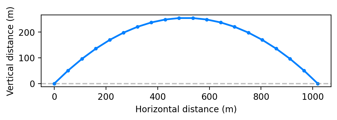
To make this a bit more tangible, we will demonstrate this with an example.

Example #

To work through an example we will first have to define the initial conditions. Suppose we want to fire a projectile starting at the origin with an angle of $\pi / 4$. The initial velocity of the projectile is 100 meters per second, and the gravitational force is 9.81 meters per second squared.

First we define all the constants, the acceleration vector, and the velocity vector.

1g = 9.81
2a = np.array([0, -g])
3angle = math.pi / 4
4force = 100
5vx = force * math.cos(angle)
6vy = force * math.sin(angle)
7v = np.array([vx, vy])

Then we calculate the displacement at increasing values of $t$. Using formula (8), we find that the moment of impact is when $t$ is $100 \sqrt 2 / 9.81$. We use this to calculate a bunch of points along the trajectory which we will plot.

1T = np.linspace(0, 2 * force * math.sin(angle) / g, 100)
2x, y = zip(*[0.5 * a * (t * t) + v * t for t in T])

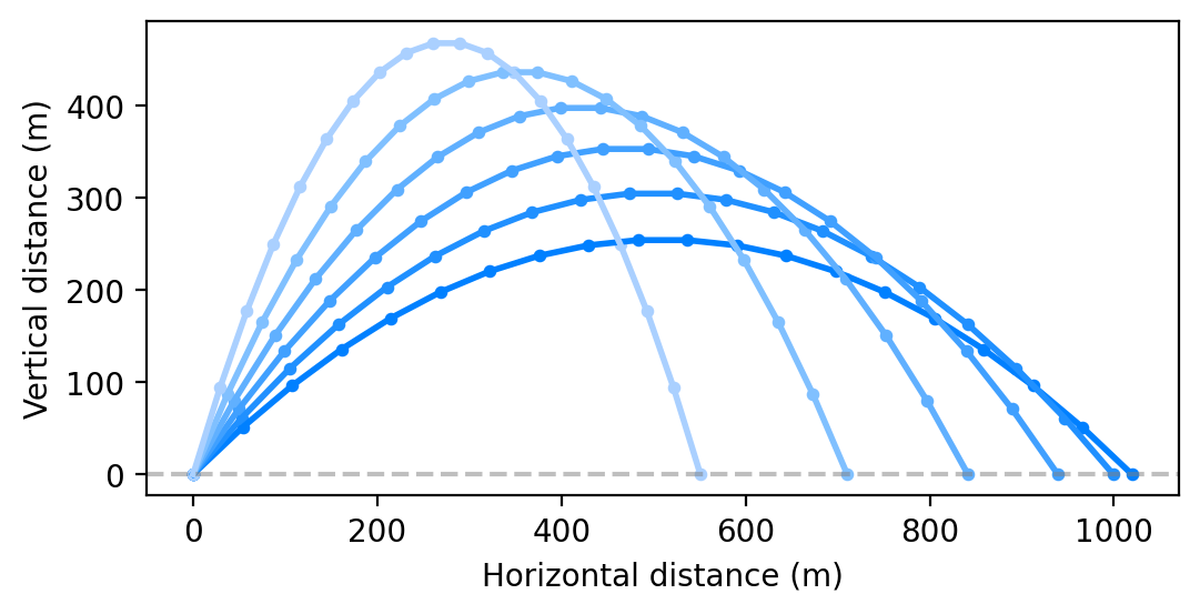
Maximum reach #

It is interesting to note that the angle $\pi / 2$ is the angle that gives the maximum distance that the trajectory can reach. If we increase the angle even further, we can see that the horizontal distance is decreasing, and the vertical distance is increasing. The plot below shows a few trajectories starting at the angle $\pi / 2$.

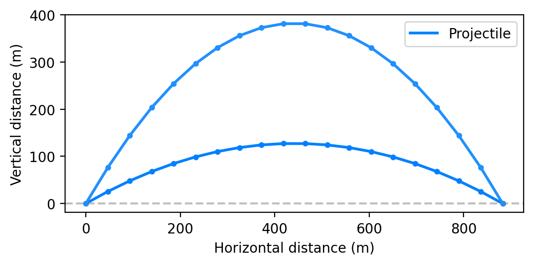
Two trajectories #

Another interesting observation is that, unless we shoot directly up, or at the angle $\pi / 2$, there are two trajectories that impact at the same point.

In the next post we will be looking at finding the angle of elevation.